In Fastai 2018 Part 2’s lesson 9, a Single-Shot Detector (SSD) is trained on the Pascal-VOC dataset for multi-object detection: to draw rectangular boxes that just fit around recognised objects . This article aims to look at the process of going from the model’s output activations to the loss in a bit more detail.
Ground-truth
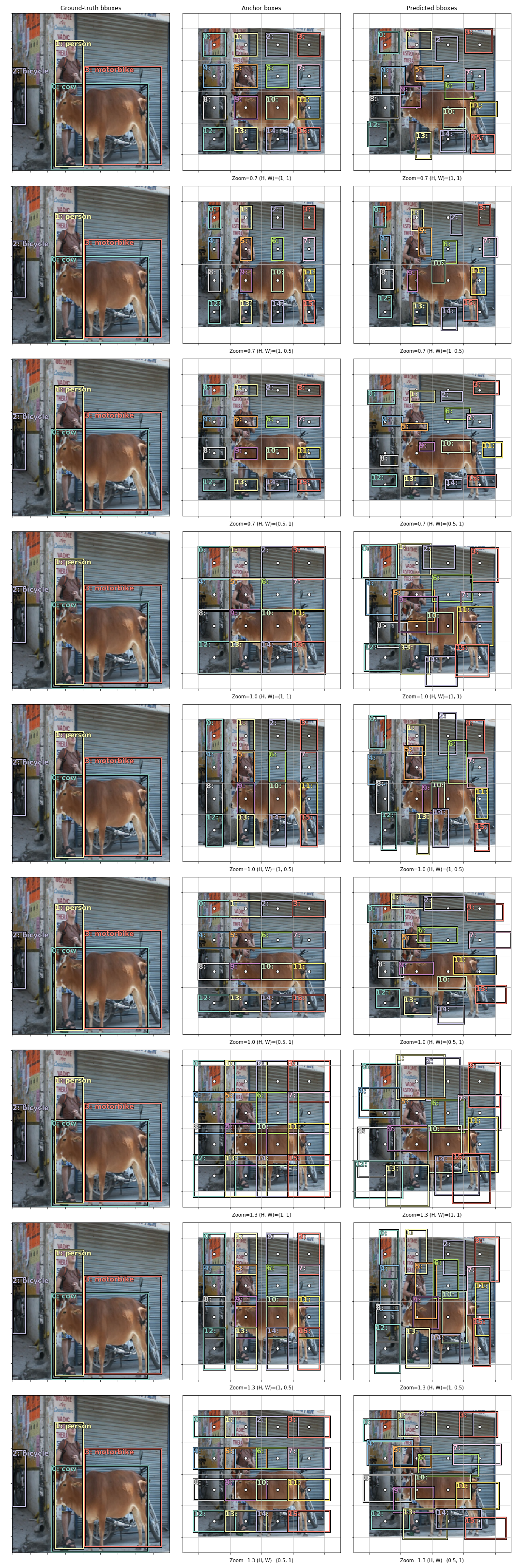
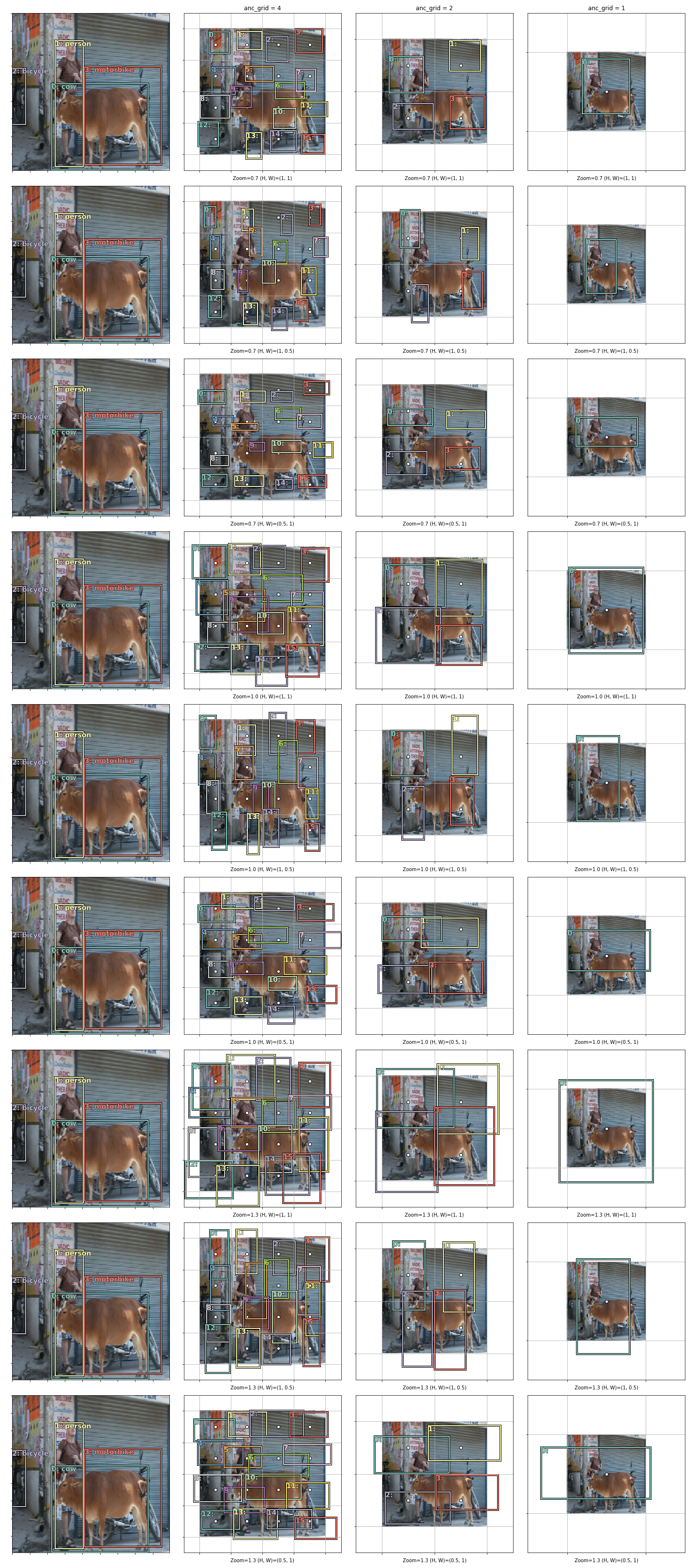
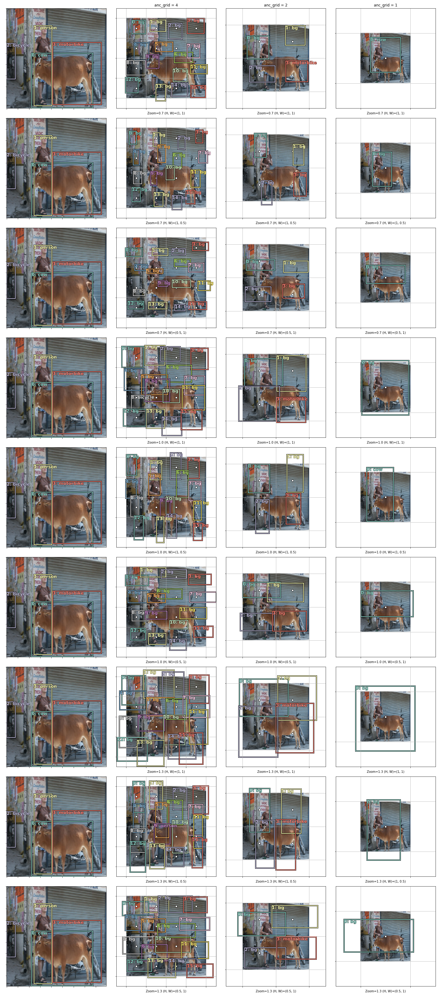
In the top-left plot of Fig.1 (below) is shown the example image that will be considered here. There is a cow, a person, a bicycle and a motorbike in it. These are the objects in the image. Just around each of them is drawn a bounding box, or a bbox. Since these have been annotated, they are also called the ground-truth bboxes. In the top-left corner of each bbox is a number; this indexes the bbox inside the plot, so if there are four bboxes in the plot, this index goes from 0 to 3. Next to the index, separated by a colon, is the class category for the object inside the bbox. Since this also has been annotated by someone, it will be referred to as the ground-truth class category. Together, the ground-truth bbox and the ground-truth class category make up the “label” (or the “y”) of this supervised learning problem, with the image being the input (or the “x”).
Height and width of model output
In this example, the input image is \(224\times224\) pixels, and the model architecture used means that the activation from the last three layers are output, where the third last layer is \(4\times4\) pixels, the second last layer \(2\times2\) pixels, and the last layer \(1\times1\) pixels.
Grid cells
The calculation of the loss begins with the construction of grid cells. Taking the third last layer as an example, because its activation is \(4\times4\), a \(4\times4\) grid is placed over the image. In the top-middle plot of Fig.1, this grid is marked out by the thin, white lines that run across the image vertically and horizontally. Each of the small square boxes in this grid is a grid cell. Using the concept of the effective receptive field, each grid cell is said to be responsible for “looking at” the part of the image inside it. In this way, the size of the grid cell is characteristic of the size of the objects that it can detect.
Anchor boxes
The centre of each grid cell is called the anchor. In the top-middle plot of Fig.1, the anchors are plotted as small white dots. About each anchor, there is drawn a square box. This is an anchor box. In this plot, the anchor boxes have a zoom of \(0.7\) and a height-width aspect ratio of \((1, 1)\), as indicated in the plot’s x-axis label. This means that the anchor box is drawn by first scaling both the grid cell’s height and width by \(0.7\), then scaling them separately by \(1\) and \(1\). One plot down, the anchor boxes have a zoom of \(0.7\) and a height-width aspect ratio of \((1, 0.5)\), making them small rectangles that appear oriented vertically. Note that in this plot, the grid cells are the same as the ones in the plot above, just that anchor boxes with a different zoom and aspect ratio are drawn. In the model considered here, 9 combinations of zoom and aspect ratio are used, so 9 anchor boxes are constructed from each grid cell. To avoid overcrowding the plot, these 9 anchors boxes are plotted separately in each of the 9 plots in Fig.1’s middle column.
Predicted bboxes
In the next step, each anchor box is reshaped and made to "float" about the anchor. The centre of the anchor box is moved to another point inside the grid cell, and its height and width are separately scaled further, to a value between .5 and 1.5 times the height/width of the grid cell. This resulting box is called the predicted bbox. For example, anchor box 11 in the top-middle plot becomes a flat rectangle whose centre is to the right of the anchor in the top-right plot after this transformation. Predicted bbox 5 shows that it is possible to "float" into a neighbouring grid cell. How much an anchor box should float away from its centre and how its height and width should be scaled is determined by the output activation, the slice associated with the grid cell. Since activations are dependent on the model weights, as the SSD receives more training, the predicted bboxes will be located and shaped closer to a ground-truth bbox. On the other hand, anchor boxes' location and shape are hardwired and do not change with training. It should be pointed out that, in the second and third columns of Fig.1, the image appears smaller because of a white margin around it. This is simply to enable parts of boxes that are outside the image to be seen. The plot of the ground-truth is repeated in the first column, for easy comparison with the other columns.
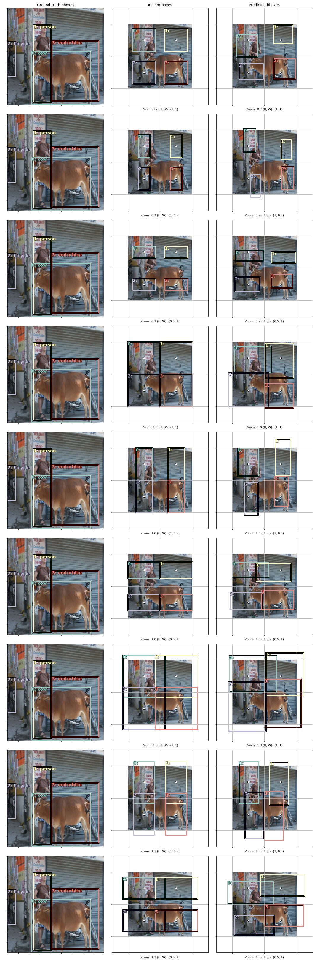
Fig.1 shows the grid cells, anchors, anchor boxes and the predicted bboxes for the third last layer of the SSD model, which has a 4x4 activation. The same things are shown in Fig.2 for the second last layer, which has a 2x2 activation. Notice that the only difference is that the boxes are larger in general. (With a larger width/height, the predicted boxes can now potentially drift farther outside the image, so a larger margin is intentionally left around the image in the plots. This has nothing to do with the SSD model. The image has not been shrunk by the SSD! )
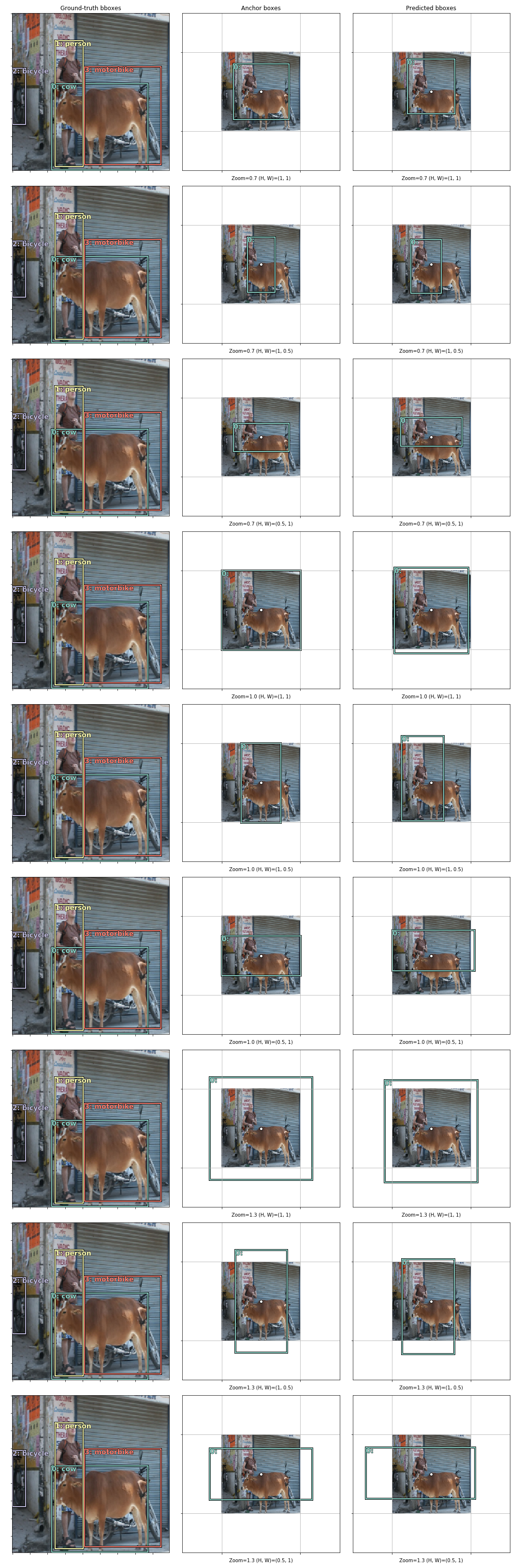
Fig.3 shows the same things, but for the last layer, which has a \(1\times1\) activation. In this case the characteristic size of the boxes is same as the size of the image.
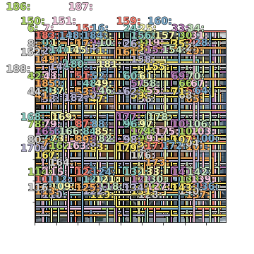
Aside. If all the anchor boxes from Fig.1-3 are overlaid on top of the image, it looks like:
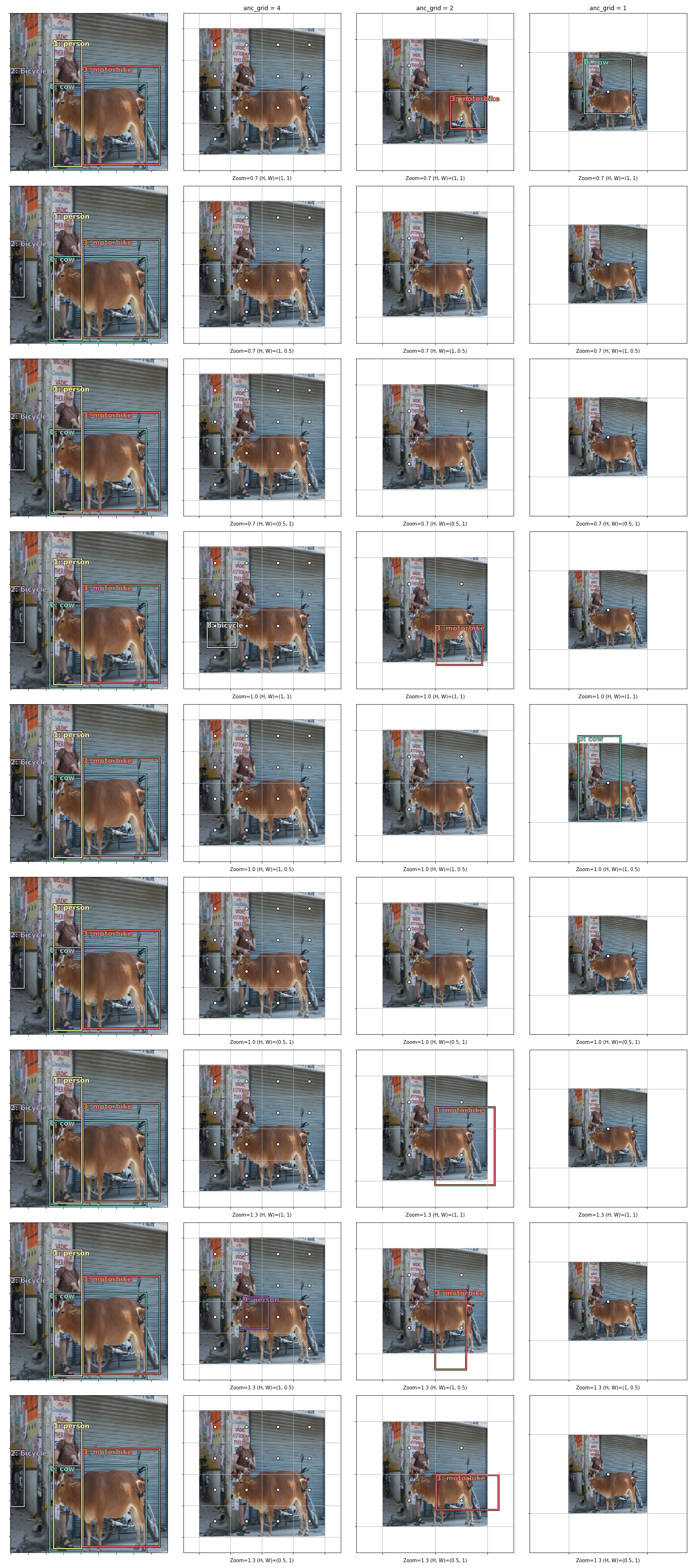
The anchor boxes are no longer needed once the predicted bboxes are obtained. In Fig.4 below, the predicted bboxes from all three output layers are gathered (from column 3 of Fig. 1–3) and shown next to the ground-truth.
Intersection-Over-Union
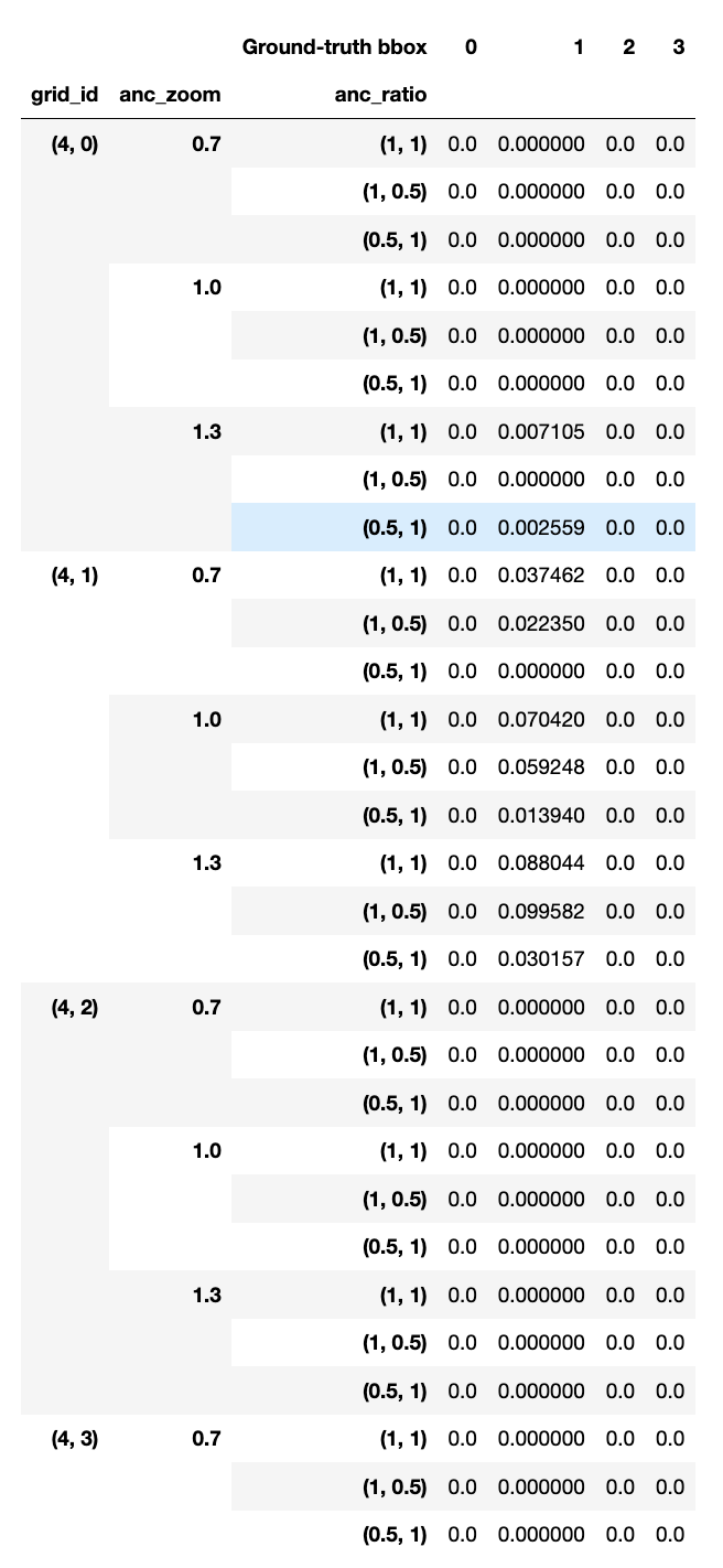
Next, the intersection-over-union (IOU) is calculated between the ground-truth bboxes and the predicted bboxes. Table.1 below shows 30 predicted bboxes’ IOUs with the ground-truth bboxes. Each row corresponds to a predicted bbox, and each column to a ground-truth bbox. Since there are 189 predicted bboxes and 4 ground-truth bboxes, there are a total of \(189\times4=756\) IOU values.
Max IOU
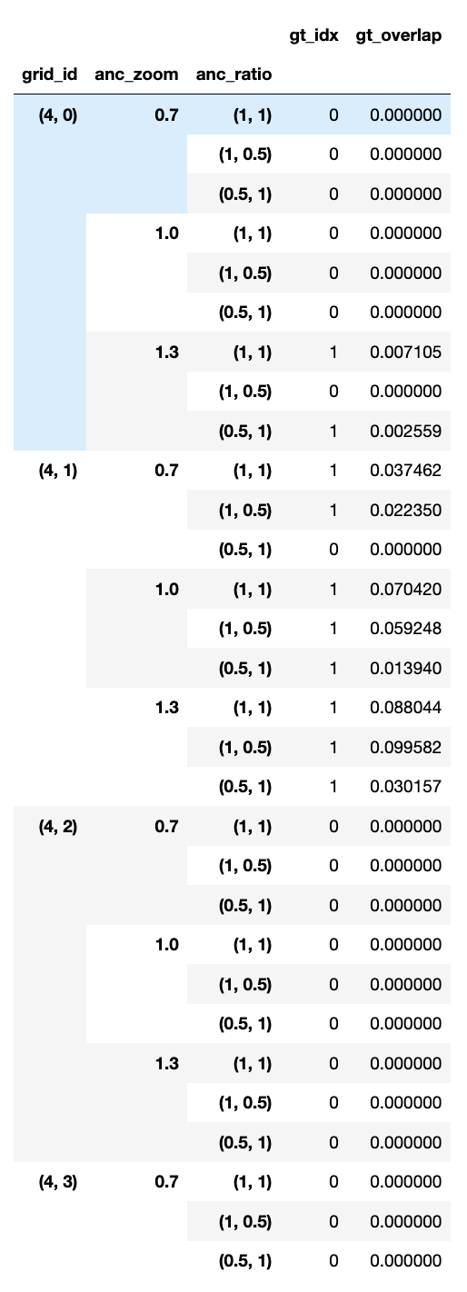
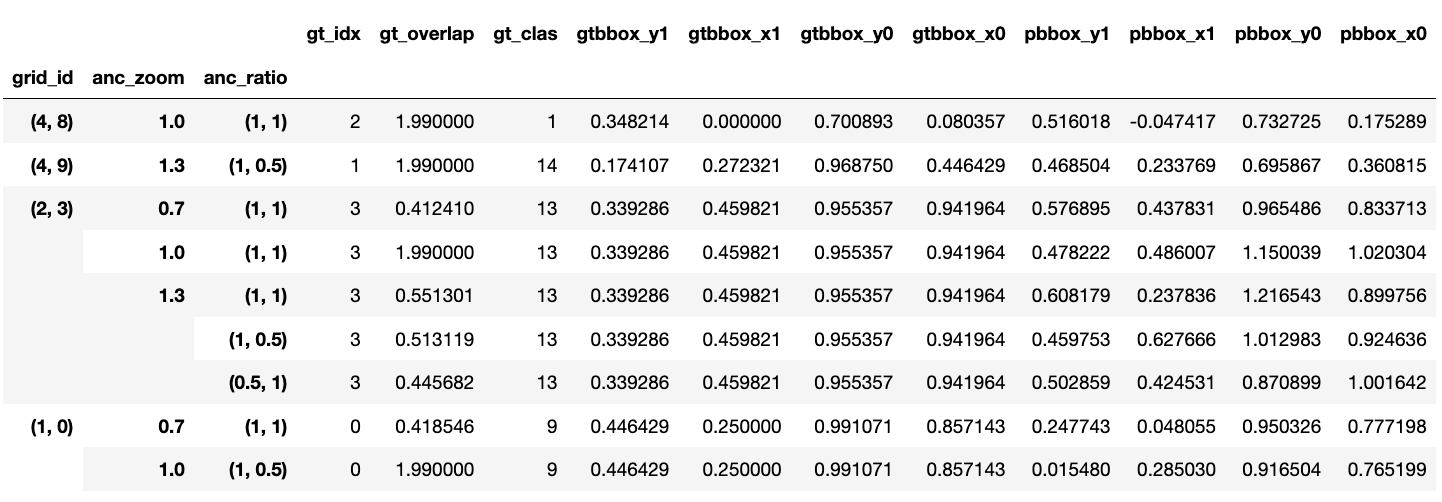
For each predicted bbox, the ground-truth bbox that it has the largest IOU with is identified, and the IOU value recorded. Table 2 shows the box index and IOU of this ground-truth bbox for 30 of the predicted bboxes. For each predicted bbox, gt_idx is the box index, and gt_overlap is the IOU value. There are two exceptions in this process however. The first one is that if a predicted bbox doesn’t actually overlap with any ground-truth bbox, the box index is nevertheless set to 0, by default. The other exception is that, in order to ensure that every ground-truth bbox is taken on by at least one predicted bbox with which it has overlap, the reverse of the above is done: for each ground-truth bbox, find the predicted bbox with which it has the largest IOU. Then, this predicted bbox’s box index in Table 2 is replaced with the box index of the ground-truth bbox here, and its IOU is nudged to 2. For example: a predicted bbox overlaps with ground-truth bboxes 0 and 1, with its IOU with 0 being larger than with 1, but because it has a larger IOU with 1 than any other predicted bbox, we actually set its box index gt_idx to 1 (instead of 0) and its IOU gt_overlap to 2.
Ground-truth class category for a predicted bbox
The next thing that is done is to give each predicted bbox a ground-truth class category, and here this is simply defined to be the ground-truth class category of the ground-truth bbox with which the predicted bbox has the largest IOU.
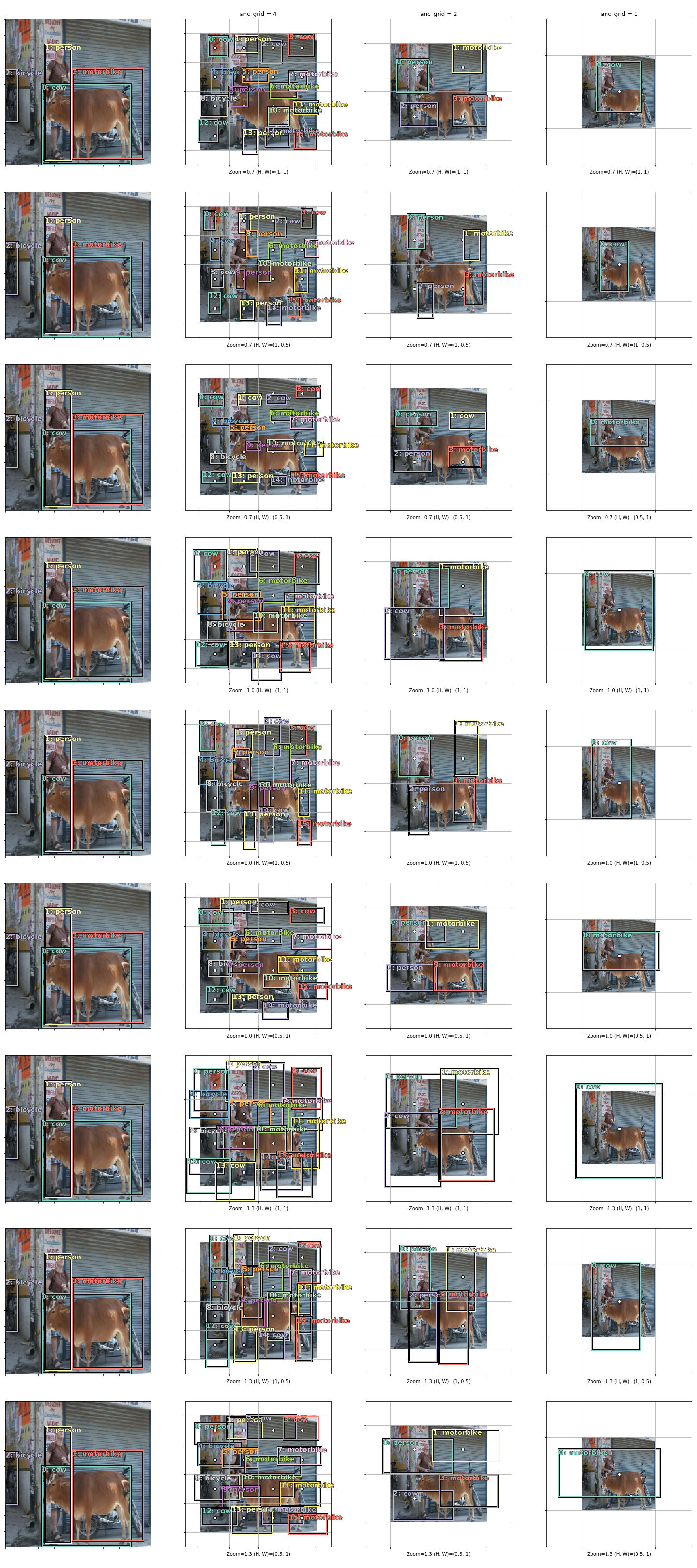
In Fig.5, the ground-truth class category label for each predicted bbox obtained this way is shown. Notice that because ground-truth bbox 0 contains a cow, those predicted bboxes that are exceptions because they don’t overlap with any ground-truth bbox have “cow” as their ground-truth class label. For example, bboxes 0, 2 and 3 in the first plot of the second column.
Adding the “background” class category
Next, we change the ground-truth class category to “background” for a predicted bbox if its IOU is less than 0.4. This not only corrects those predicted bboxes that originally had no overlap at all, but also those predicted bboxes that really didn’t contain much of an object. For example, in the first plot of the second column in Fig.5, predicted bbox 1 has the ground-truth class category “person”, but it’s clear that, by comparing with the ground-truth plot to the left, it only has a tiny bit of an overlap with the “person” ground-truth bbox, and the rest is just “background”. Doing this, many predicted bboxes now have “background” as its ground-truth class category, as seen in Fig.6.
At this point, we are in a position to calculate the loss due to classification and the loss due to regression, and they can be done separately.
Classification Loss
For this, each predicted bbox is effectively treated as an image in itself and the problem becomes a single-label classification problem. For each predicted bbox, or grid cell, the output activation contains 21 numbers, each of which represents the probability of each possible class category. For example, if the probability for the “car” class category is 0.3, then it means that the model thinks there is a 30% chance that whatever is inside the predicted bbox is a car. Using these probabilities and the ground-truth class category of the predicted bbox, the binary cross entropy loss is calculated. Summing this over all predicted bboxes gives the total loss due to classification for this image.
Regression Loss
For the loss due to the location and extent of the predicted bboxes, the predicted bboxes whose ground-truth class category is “background” are ignored. With this criterion, only 9 remains in this example. Each of the remaining predicted bboxes is compared with the ground-truth bbox with which it has the largest IOU.
Each box, whether it is a predicted bbox or a ground-truth bbox, is described by four numbers, \((y_0,x_0,y_1,x_1)\): the \(x\) and \(y\) coorindate values of the top-left and bottom-right corners. In Table 4 below, \(y_0\) and \(x_0\) are the coordinates for the top-left corner, and \(y_1\) and \(x_1\) are the coordinates for the bottom-right corner. gtbbox is for ground-truth bbox; pbbox is for predicted bbox. Notice that there are now only 9 rows in the table because only 9 predicted bboxes remain.
The mean absolute error from these four numbers is calculated for each predicted bbox. Summing this over all predicted bboxes gives the total loss due to bbox regression for this image.
SSD Loss
Finally, the sum of the classification and regression loss is the SSD loss, from which the back propagation starts.
You can find the notebook I used for this post at: https://github.com/qAp/fastai/blob/mywork/courses/dl2/pascal-multi-dissected.ipynb.
