Satellite image resolution
The spatial resolution of a satellite image is usually specified as the distance on the ground covered by a pixel in the image. At 0.3 m resolution, each pixel covers a distance of 0.3 m. Say a car is about 3 m long, then in such an image, about 10 pixels span the length of the car.
If the image is at 0.1 m resolution, then there are about 30 pixels that span the car. Since a pixel is a unit of information in an image, the more pixels there are that span an object, the more details that can potentially be revealed about the object.
Super-resolution
Suppose the only images that are available to begin with are at 0.3 m resolution, but it is desirable to have larger images, say at 0.1 m resolution — an increase by a factor of 3. Linear, bilinear, or bicubic interpolation can be used to enlarge the images by a factor of 3. However, the resulting images using these methods tend to be quite blurry, which doesn't help much. Super-resolution refers to a class of more sophisticated techniques for increasing image resolution that produces better results.
In the context of supervised learning, having high resolution images that reveal more content details allows for easier and better data annotation, such as for object detection or segmentation, because more pixels and more details can be packed into the same area on the computer screen. Training a computer vision model with a larger image size can potentially increase the model's performance as well.
Super-resolution models
Many super-resolution models increase the resolution by an integral factor, called the scale factor. For example, the scale factor is 3, in going from 0.3 m resolution to 0.1 m resolution. In this case, the image width and height are increased by a factor of 3, and the image area is increased by a factor of 9.
Models are typically trained by showing them examples of image pairs, in which both images are the same except that one's resolution is larger than the other's by a factor equal to the model's scale factor. The image with lower resolution is called the low resolution (LR) image, while the other is called the high resolution (HR) image. The output image of the model is often referred to as the super-resolved (SR) image. Effectively, the model is trained to produce SR images that are as close to the HR images as possible.
ESRGAN
The Enhanced Super-resolution Generative Adversarial Network (ESRGAN) is a nerual network architecture for single image super-resolution. It's an enhanced version of the Super-resolution Generative Adversarial Network (SRGAN), one of the first super-resolution neural networks to use perceptual loss. These neural networks generate realistic-looking SR images.
Compared with the SRGAN, the ESRGAN differs in that the generator network has all the batch normalisation layers removed, because these are believed to be responsible for unpleasant artifacts in the SR images, especially when the test set is statistically different from the train set and when the networks are deeper. Therefore, removing batch normalisation should improve the generalisability of the model. The ESRGAN generator also has more residual connections, which increases the "network capacity".
Relativistic average discriminator
For the adversarial loss, the ESRGAN authors use the relativistic average discriminator: $$ D(x, S) = \sigma \left( C(x) - \frac{1}{|S|} \sum_{x' \isin S} C(x') \right) $$ Here, \(x\) denotes an image. \(C(x)\) is the output score of the discriminator network on the image \(x\). \(S\) denotes a set of images. And \(\sigma\) is the sigmoid activation function. \(D\) measures the discriminator output score of the image \(x\) relative to the average score for the set of images \(S\). It's in the range \((0, 1)\). The closer to 0 it is, the smaller \(x\)'s output score is relative to the scores in \(S\). The closer to 1 it is, the larger \(x\)'s output score is relative to the scores in \(S\).
Suppose \(S\) is a mini-batch consisting of SR and HR images, then $$ S = S_r \cup S_f $$ where \(S_r\) are the HR images in the mini-batch, and \(S_f\) are the SR images in the mini-batch. The subscript \(r\) stands for 'real', and the subscript \(f\) stands for 'fake'. Because the SR images are images produced by the generator network, they are the fake images, as opposed to the real, original HR images.
Suppose the discriminator's adversarial loss is defined as: $$ L_D^{Ra} = \frac{1}{|S_r|} \sum_{x \isin S_r} -\log[D(x, S_f)] + \frac{1}{|S_f|} \sum_{x \isin S_f} -\log[1 - D(x, S_r)] $$ Then, in minimising it, \( D(x, S_f) \) tends to 1 for real images and \( D(x, S_r) \) tends to 0 for fake images. This in turn means that the output scores of the real images becomes larger than the output scores of the fake images, or \(C(x_r) > C(x_f)\). The definition for the generator's adversarial loss follows from this: $$ L_G^{Ra} = \frac{1}{|S_r|} \sum_{x \isin S_r} -\log[1 - D(x, S_f)] + \frac{1}{|S_f|} \sum_{x \isin S_f} -\log[D(x, S_r)] $$ For the generator, the opposite behaviour is desired. Since, for the discriminator, \( D(x, S_f) \) tending to 1 is desired, for the generator, \( D(x, S_f) \) tending to 0 is desired instead. Same logic applies to \( D(x, S_r) \).
The reason for using the relativistic average discriminator \( D \) is that now the generator can take advantage of the gradient contribution from the fake data as well as the real data. In SRGAN, there is only contribution from the fake data.
Training procedure
Whilst the total loss for the discriminator is just the adversarial loss \(L_D^{Ra}\), for the generator, there are 2 additional losses: $$ L_G = \epsilon L_{percep} + \lambda L_G^{Ra} + \eta L_1 \quad, $$ namely, the perceptual loss \( L_{percep} \), and the \(L_1\) loss. The training happens in 2 stages.
In the first stage, \(\eta = 1\) and \( \epsilon = \lambda = 0 \). In this stage, the training concentrates on getting a pixelwise agreement between the HR and the SR image. Since this optimises what's called the PSNR metric, the resulting generator from this stage is called the PSNR-oriented network, \(G_{PSNR}\).
Following this, in the second stage, \(\eta\), \(\epsilon\), and \(\lambda\) are all non-zero. The actual adversarial training takes place in this stage. The resulting generator is called the GAN-based network, \(G_{GAN}\).
Doing the stage 1 training before the adversarial training allows the generators to avoid undesired local optima, and it provides the discriminator with images that already have quite a good resolution in stage 2, which helps it to focus more on texture discrimination.
During inference, the parameters of the model used are the weighted averages of those from the \(G_{PSNR}\) and the \(G_{GAN}\).
More details about the ESRGAN, its architecture and training procedure, can be found in its official paper ESRGAN: Enhanced Super-Resolution Generative Adversarial Networks.
There are several implementations of the ESRGAN available on Github, one of which is ESRGAN-pytorch: https://github.com/wonbeomjang/ESRGAN-pytorch, the one used in this post.
Super-resolving satellite images
Suppose there is a set of satellite images at 0.6 m resolution, and the task is to increase their resolution (these images will be referred to as the target images, for clarity).
Training dataset
The pre-trained ESRGAN models provided by ESRGAN-pytorch can be applied to these images to increase their resolution. Like most ESRGAN implementations out there, and as described in the original paper, these models have been trained on the DIV2K and Flickr2K datasets, which contain high fidelity, natural images, such as those taken of everyday objects by consumer digital cameras. These pre-trained models may therefore not be ideal for satellite images, which are taken from aerial views and by instruments having optics quite different from those in consumer cameras, so some training on satellite images is likely required.
The bigger increase in resolution that is desired, the larger the scale factor that is needed, but 4 is a good value if it's sufficient, since that is the scale factor most ESRGAN models have.
If the ESRGAN is to be trained, or fine-tuned, on satellite images, simply taking the target satellite images as the HR images for training is probably not a good idea, because it seems this way the most that can be expected is something that's only as good as the target images themselves. A rectangular patch on the road is still, at best, seen as a rectangular patch, and not a car, because there's no extra information there to suggest that there is a windscreen. Therefore, it seems that the HR images for training should have a higher spatial resolution than the target images.
At how much higher a spatial resolution then? It would seem natural to deduce from the scale factor of 4 that the HR images which need to be collected for training should have a resolution that is 4 times greater than the target images. But this might not be strictly necessary. After all, in the natural images in DVI2K, surely a cat can appear larger in some pictures than in some others, because the camera was closer. So, if all the HR images are at a resolution exactly 4 times higher, then a car would always be exactly 4 times longer than in the LR images. Having HR images at various different resolutions might provide more complexity for the model to learn.
Different parts of the world can look quite different from the air, so idealy the training images should come from a variety of locations.
For the results presented here in this post, the dataset of training images consists of some images of Paris, Las Vegas, and Khartoum, at 0.3 m from Spacenet V2, of Wellington at 0.1 m from Land Information New Zealand.
Crops of size 128 px \(\times\) 128 px are taken from all these images; these crops are the HR images used during training. All images are then scaled down by a factor of 4 in length, and corresponding crops of size 32 px \(\times\) 32 px are taken from these, which are the LR images used during training. The ratio of the sizes of HR and LR images here correspond to a scale factor of 4, the same as the pre-trained models.
Training procedure
ESRGAN-pytorch comes with two pre-trained models: \( G_{PSNR} \) and \( G_{GAN} \) — the resulting generators from stage 1 and stage 2 training (as described in the ESRGAN section), respectively.
It seems logical to make use of these, because they have been trained for a large number of iterations on a large number of high fidelity images. What is not clear immediately is how these should be fine-tuned with the satellite images. Should the starting parameters be those from \( G_{PSNR} \) or \( G_{GAN} \), and should stage 1 or stage 2 training be used in the fine-tuning, or both, with one following the other? And how many epochs of training should be done?
After trying some of these options, what does not seem to work well is to carry out stage 1 training followed by stage 2 training on the satellite images, whether the starting point is \( G_{PSNR} \) or \( G_{GAN} \). Maybe this is because the satellite images are simply not complex enough in terms of textures, angles of views, colours, and shapes, and so training on them for too long wipes out too much of what has been learnt from the DIV2K images, as the resulting SR images are quite blurry.
Based on how the resulting SR images look, it seems that the best option is to start with \( G_{GAN} \) and only do stage 2 training. A plausible explanation is that because \( G_{GAN} \) is the final product of training on DIV2K, so it has learnt more from DIV2K than \( G_{PSNR} \), and since stage 1 training is really regarded by the authors as a 'pre-training' step, it's probably sufficient to have already done it on DIV2K.
Results
In comparing images in the context of super-resolution, it helps to keep in mind that the HR and SR images have the same size, and they are larger than the LR images and so have more pixels. If each image pixel is displayed over an area of the same size, on a computer screen or on a piece of paper, not only do the HR/SR images appear larger than the LR images, due to the extra pixels they have, more information or details might also be revealed about the content of the image. At the same time, if the HR/SR images and the LR images are made to fit inside an area of the same size, the HR/SR images can appear "sharper" than the LR images, because more pixels are packed inside the same area.
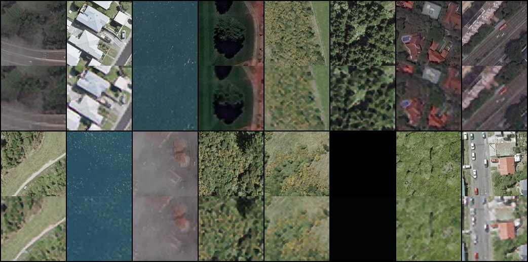
As described above, starting with parameters from \(G_{GAN}\), stage 2 (GAN-based) training on the satellite images collected is carried out. It's interesting to compare the HR and SR images early in the training process, because at this stage \(G_{GAN}\) has seen very few satellite images. It is seen that, after just 1 epoch, the SR images look somewhat blurry compared with the HR images, but it's possible to make out the overall composition.
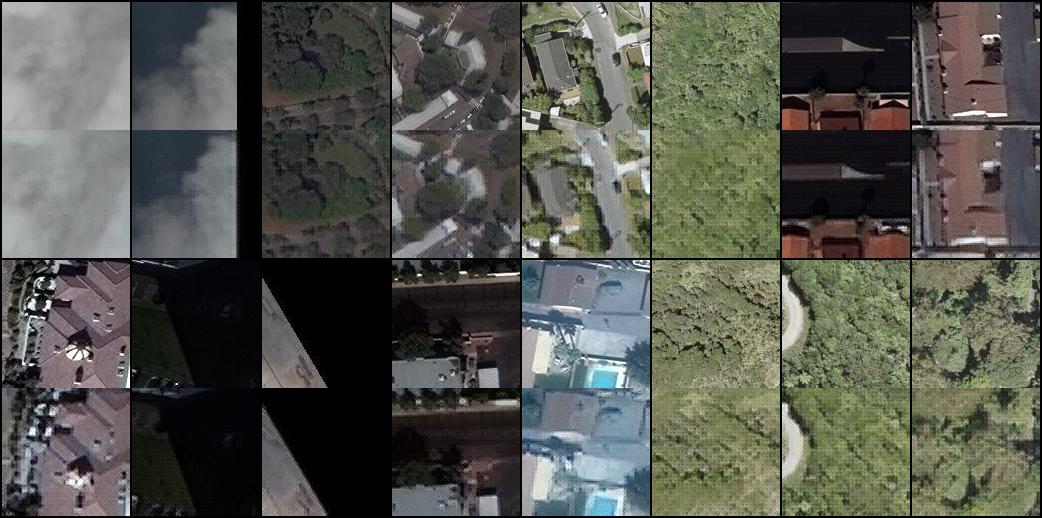
After a further 107 epochs of training, the SR images now look 'sharper' than they are after just one epoch, but at the same time, there is a fake-looking, dotted texture to them. Thin lines are still not visible. Let this generator that has gone through training on the satellite images be denoted by \(G_{GAN,sat}\).
In the ESRGAN paper, at test time, the following network interpolation is used to obtain realistic, high fidelity SR images:
$$ G = 0.2 G_{PSNR} + 0.8 G_{GAN} $$
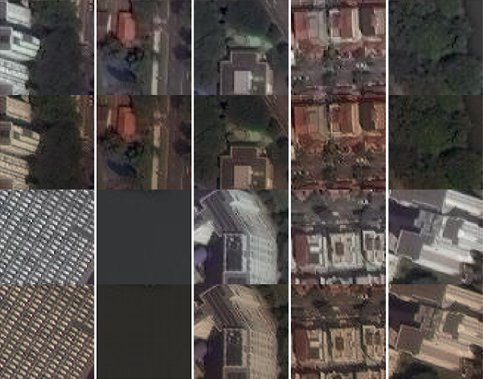
Applying \(G\) to the target images, it can be seen that there is less pixelation in the SR images than in the LR images. The colours in the SR images seem a bit too warm compared with the LR images. This might be due the difference in the data distributions of DIV2K and the satellite images.
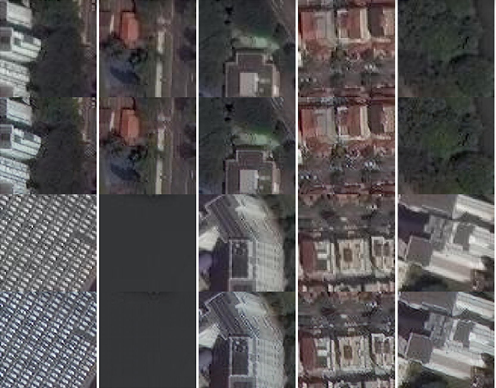
With some training on the satellite images, it can be seen that the colours appear to be closer to the LR images'. Although overall, it's probably fair to say that the SR images do not appear that much sharper, nor do they reveal extra details about the objects in the images, at least to the naked eye. However, they are 4 times larger in size than the LR images, and so they can still potentially provide improvement on some other computer vision task, when used as the training examples in place of the LR images.
See here for my fork of ESRGAN-pytorch, which has distributed paralell and mixed-precision training enabled, and notebooks containing examples of training and inference.