Grad-CAM in Deepfake Face Recognition

Class activation mapping (CAM) can be thought of as an interpretation tool for convolutional neural networks. It visually explains the prediction made by the neural network by highlighting certain areas in the input image. These areas are said to have been looked at most 'closely' by the neural network in making its prediction.

In object recognition, if a model predicts 'dog' from an input image containing a person walking his dog, you expect the CAM to highlight the area centred around the dog. If the model predicts from the same image the caption 'Man walking dog'. In this case it would make sense for both the person and the dog to be highlighted in the image.

Deepfakes are these realistic-looking images or videos where a person's face has actually been artificially manipulated. There are various techniques for generating deepfakes, but in general the result is that the original face is subtly altered. What is it, then, that a neural network 'looks at' to decide that an image of a face is a deepfake? We apply a pretrained deepfake classifier to several deepfake videos and construct CAMs to see if they give an indication as to what the classifier looks at in an image to be able to tell that it's a deepfake. Along the way it's shown how Pytorch hooks are used in general to extract information from inside a model.

The model that will be used here is an EfficientNet-b1 model that has already been trained to classify an image of a face as either FAKE or REAL. It's not the best performing model out there; it forms the basis of a solution that has a logloss score of about 0.51980 on the private leaderboard of Kaggle's Deepfake Detection Challenge. (1st-place solution's score is 0.42320.)

The classifier works on images of faces, so crops of faces need to be made out of the videos to be looked at. For this, Pytorch RetinaFace is used to recognise faces in the video frames. Despite being relatively slow, it's a very accurate face recognition system.

The Kaggle Deepfake Detection challenge provides a good set of deepfake videos to work with. Each video is about 10 seconds long, and what's very useful is that the metadata shows which other video is the original version of the deepfake, so this is useful for frame-by-frame comparison. Here, several deepfake videos from the train_example_videos set of this dataset are selected, and their CAM will be looked at.

A CAM is supposed give an indication of what the model thinks as important in the image when making certain predictions, or more precisely in the current context, what it regards as important in predicting the score for an image being FAKE. As such, there are two main ingredients to consider in constructing a CAM:

1. The output activation of a convolutional layer

2. The output score for a selected class (FAKE in current example).

That the CAM should be constructed from the output activation of a convolutional layer in the model can perhaps be justified by the fact that these have spatial correspondence with the input image, and that activation in general reflects the amount of excitation, and hence 'importance', due to certain pixels (receptive field) in the image. However, the output activation alone isn't enough, because it's computed from the input image through the forward propagation; there is nothing about it that has come from the score of a predicted class of interest. To incorporate this, the gradient of the score on the output activation is used, too.

Here is how the output activation and the gradient of the output score on it are combined to form the CAM. Suppose \(A_{ij}^k\) is the output activation of one of the model's convolutional layers, where \(i\) and \(j\) are the indices for the spatial (width and height) dimensions, and \(k\) is the index for the channel dimension. And let \(y^{c}\) be the model's output score for the image being FAKE (this needs not be a probability, could be a score just before a softmax). First, the gradient of \(y^c\) on \(A^k_{ij}\) is averaged over the spatial dimensions (equivalent to applying global average pooling): $$ \alpha^{c}_{k} = \frac{1}{Z}\sum_{i}\sum_{j}\frac{\partial{y^c}}{\partial{A^k_{ij}}} $$ Since \(\frac{\partial{y^c}}{\partial{A^k_{ij}}}\) measures how fast \(y^c\) changes with \(A^k_{ij}\), \(\alpha^{c}_{k}\) is a measure of the importance of channel \(k\) for output class \(c\), and so it makes sense to use \(\alpha\) in a weighted average to reduce the channel dimension of \(A^k_{ij}\). This is essentially the CAM: $$ L^c_{ij} = ReLU\left(\sum_{k} \alpha^c_k \: A^k_{ij}\right) $$ Notice that a \(ReLU\) is applied to the weighted average over channels. In the literature, technically, the above is called the gradient-weighted class activation mapping (Grad-CAM). In the special case where \(A\) is from the last convolutional layer, and after which there is only one linear layer in the model, it's just called CAM. In principal, the above expression can be applied to any convolutional layer in the neural network to get the Grad-CAM.

\(A^{k}_{ij}\), an output activation, is computed during the forward propagation, and \(\frac{\partial{y^c}}{A^{k}_{ij}}\), a gradient, is computed during the backward propagation. The way to get at these quantities in Pytorch is to use hooks. Once a layer whose output activation is to be considered for the CAM is chosen, two hooks are attached to it: one to get \(A^{k}_{ij}\) during forward propagation, and the other to get \(\frac{\partial{y^c}}{A^{k}_{ij}}\) during backward propagation.

Below is an implementation that allows the creation of such hooks and the storing of the activation and the gradient.

class FwdHook():
    def __init__(self, m):
        self.hook_handle = m.register_forward_hook(self.hook_func)
    def hook_func(self, m, i, o): self.stored = o.detach().clone()
    def __enter__(self, *args): return self
    def __exit__(self, *args): self.hook_handle.remove()

class BwdHook():
    def __init__(self, m):
        self.hook_handle = m.register_backward_hook(self.hook_func)
    def hook_func(self, m, ig, og): self.stored = og[0].detach().clone()
    def __enter__(self, *args): return self
    def __exit__(self, *args): self.hook_handle.remove()

This implementation is taken from The Fastbook by Jeremy Howard and Sylvain Gugger. FwdHook is used for forward propagation, and BwdHook is used for backward propagation. Central to these are the register_forward_hook and register_backward_hook methods of nn.Module objects. These allow \(A_{ij}^k\) and \(\frac{\partial{y^c}}{\partial{A_{ij}^k}}\) to be accessed during forward and backward propagation, respectively. FwdHook and BwdHook also allows the accessed activation and gradient to be stored in them (as the stored attribute). They're also context managers (as defined by their __enter__ and __exit__ methods), so will safely disconnect the hooks once the things that are needed have been stored away. FwdHook and BwdHook are all but equal, except that one has forward_hook and the other has backward_hook. One other minor difference is that the gradient on the output activation, og, is a tuple, from which the first element is taken.

So now, we can attach the hooks to a selected layer of the model, pass an image through the model (forward propagation), backpropagate from the output score for the FAKE class. These steps are summed up in the following function:

def classify_face(im, cam_module):
    xb = im[None,...] / 255
    xb = xb.sub_(mean_norm[None,:,None,None]).div_(std_norm[None,:,None,None])
    xb = xb.to(device)
    model.eval()
    cls = 0
    with BwdHook(cam_module) as bwdhook:
        with FwdHook(cam_module) as fwdhook:
            output = model(xb)
            act = fwdhook.stored[0]
        output[0,cls].backward()
        grad = bwdhook.stored[0]

    gradcam = (grad.mean(dim=(1,2))[:,None,None] * act).sum(dim=0).relu_()
    with torch.no_grad(): prob = F.softmax(output[0], dim=-1)[0]
    return prob, gradcam

im is the tensor of the image of interest. cam_module is the layer (or module) of interest. The forward propagation's hook is nested inside the back propagation's because forward propagation happens first, so we will get the output activation from that, remove the forward hook, before doing the back propagation, getting the gradient, and then removing the backward book. The backward propagation is done by calling the backward method of the output score for the FAKE class, \(y^{0}\) (here \(0\) is for FAKE, and \(1\) is for REAL). It's important that the thing from which backward is called is a scalar.

Like what normally happens during inference, a single image is processed at a time, and the model is set to eval mode. However, a difference is that, here, things are not done under the torch.no_grad() context, because the gradient is needed.

After the needed quantities, \(A_{ij}^k\) and \(\frac{\partial{y^c}}{\partial{A_{ij}^k}}\), are obtained, and the hooks removed, the Grad-CAM is put together, following the description above: gradcam = (grad.mean(dim=(1,2))[:,None,None] * act).sum(dim=0)

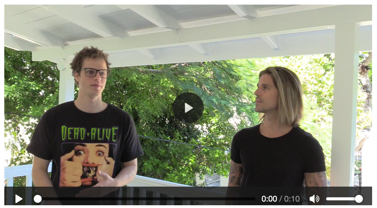
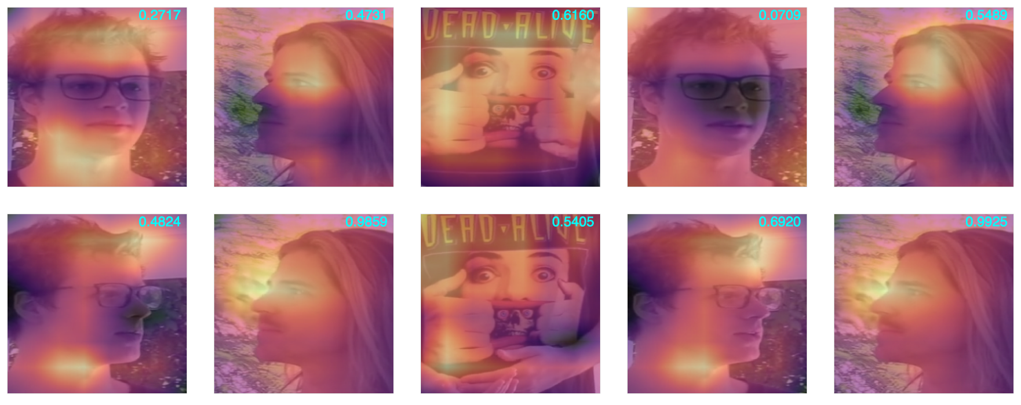
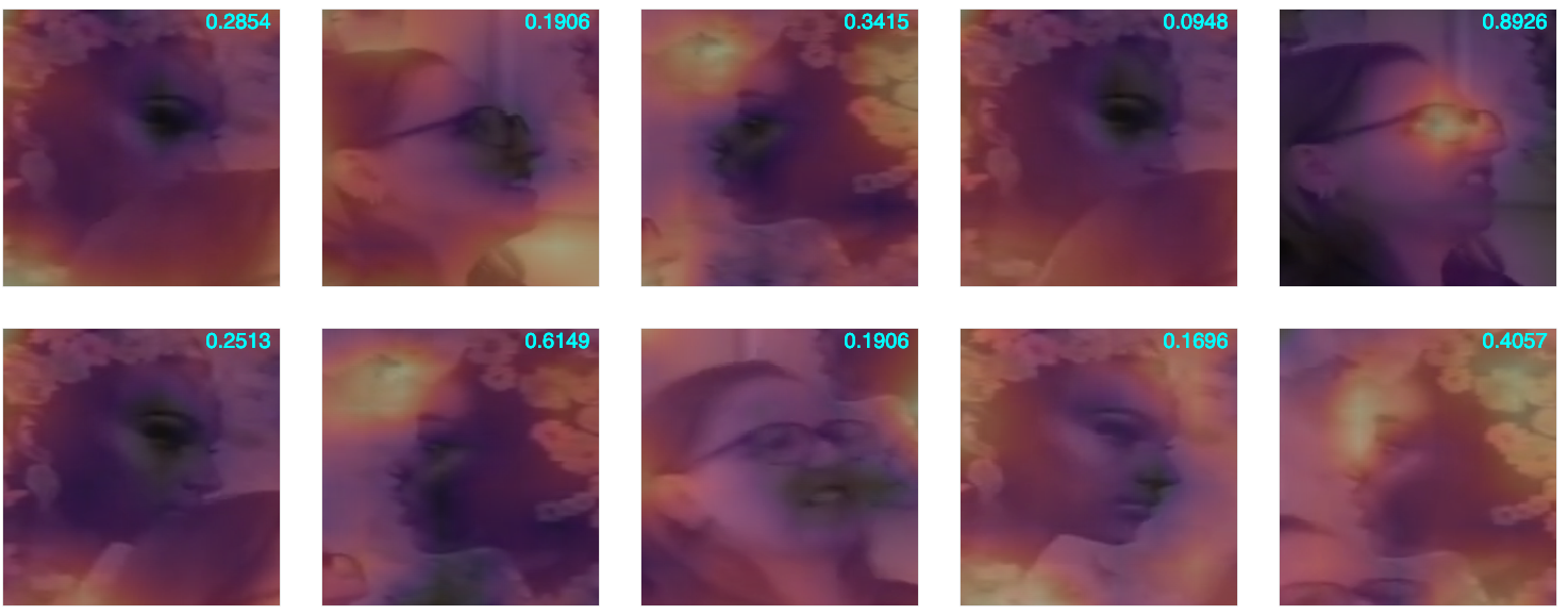
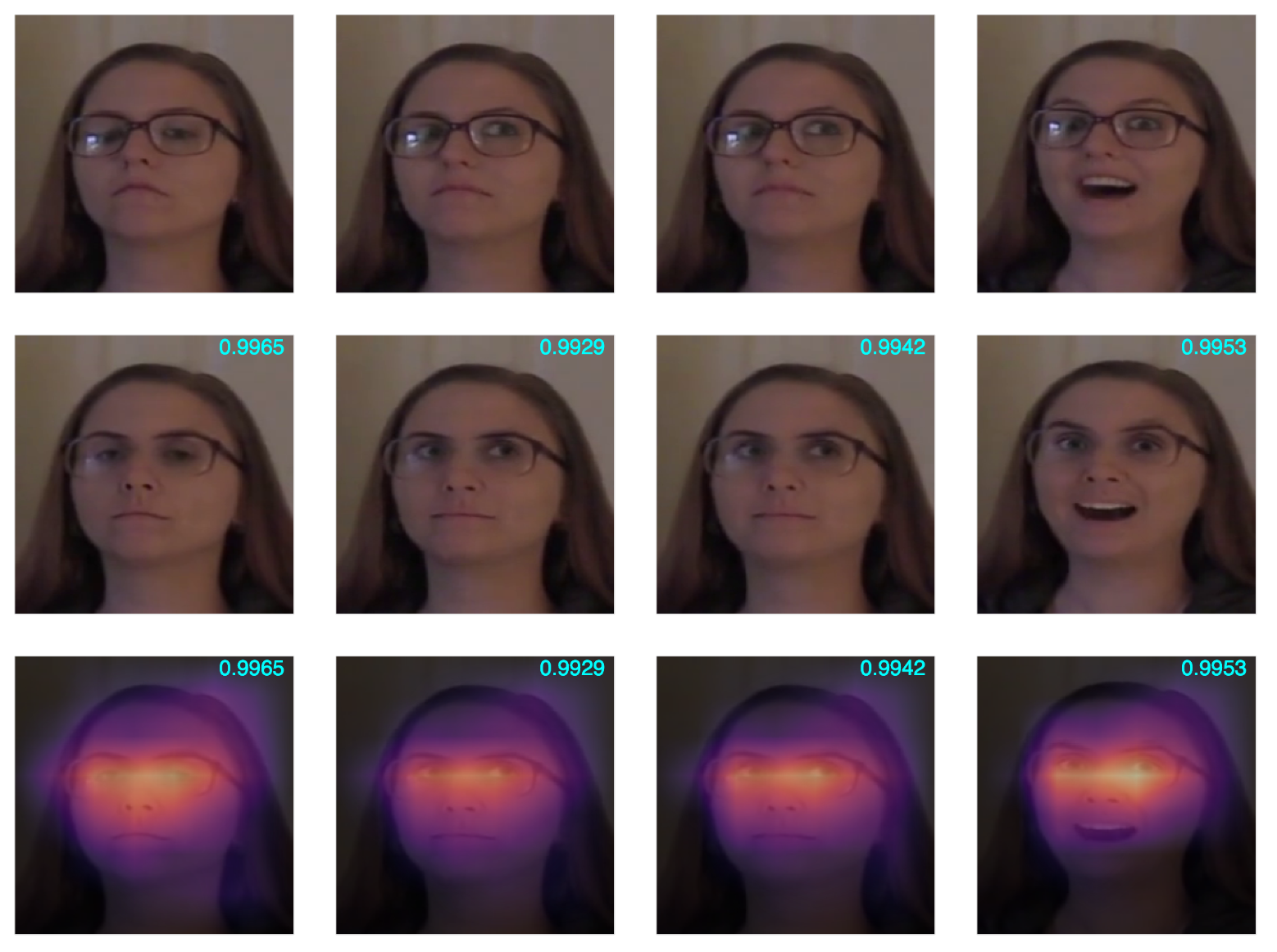
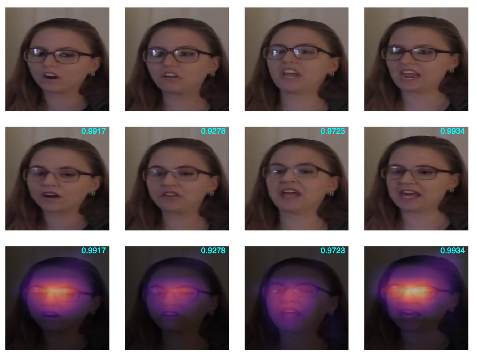
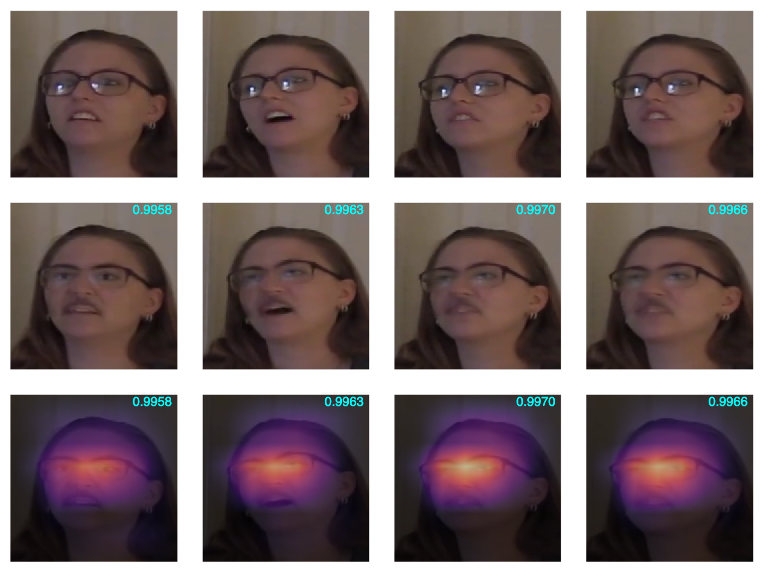
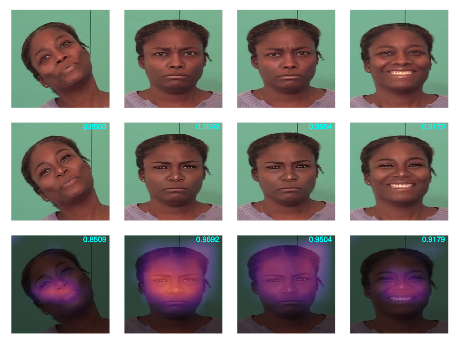
Now let's just look at the CAM of several example videos. In each example, an original video (without deepfake manipulation) and its deepfake version are used. Five frames are randomly selected from both videos, so they align, and the face is cropped from each frame. The top row in the figure shows the original faces. The second row shows the corresponding deepfake faces, and the third row shows the deepfake faces with the CAM overlaid. The CAM is plotted here with the magma colour map, so the more yellowish it is, the higher its value. In the top-right corner of the deepfake faces, the number shown is the probability with which the model thinks the face is a deepfake.

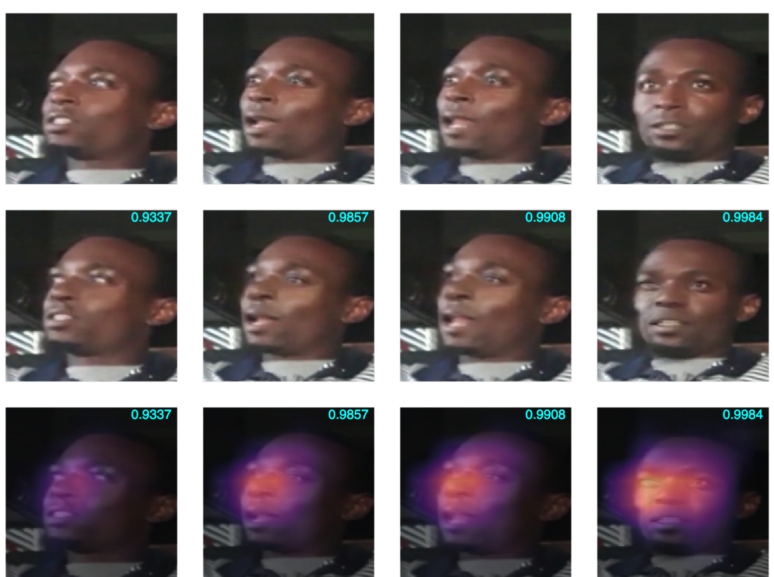
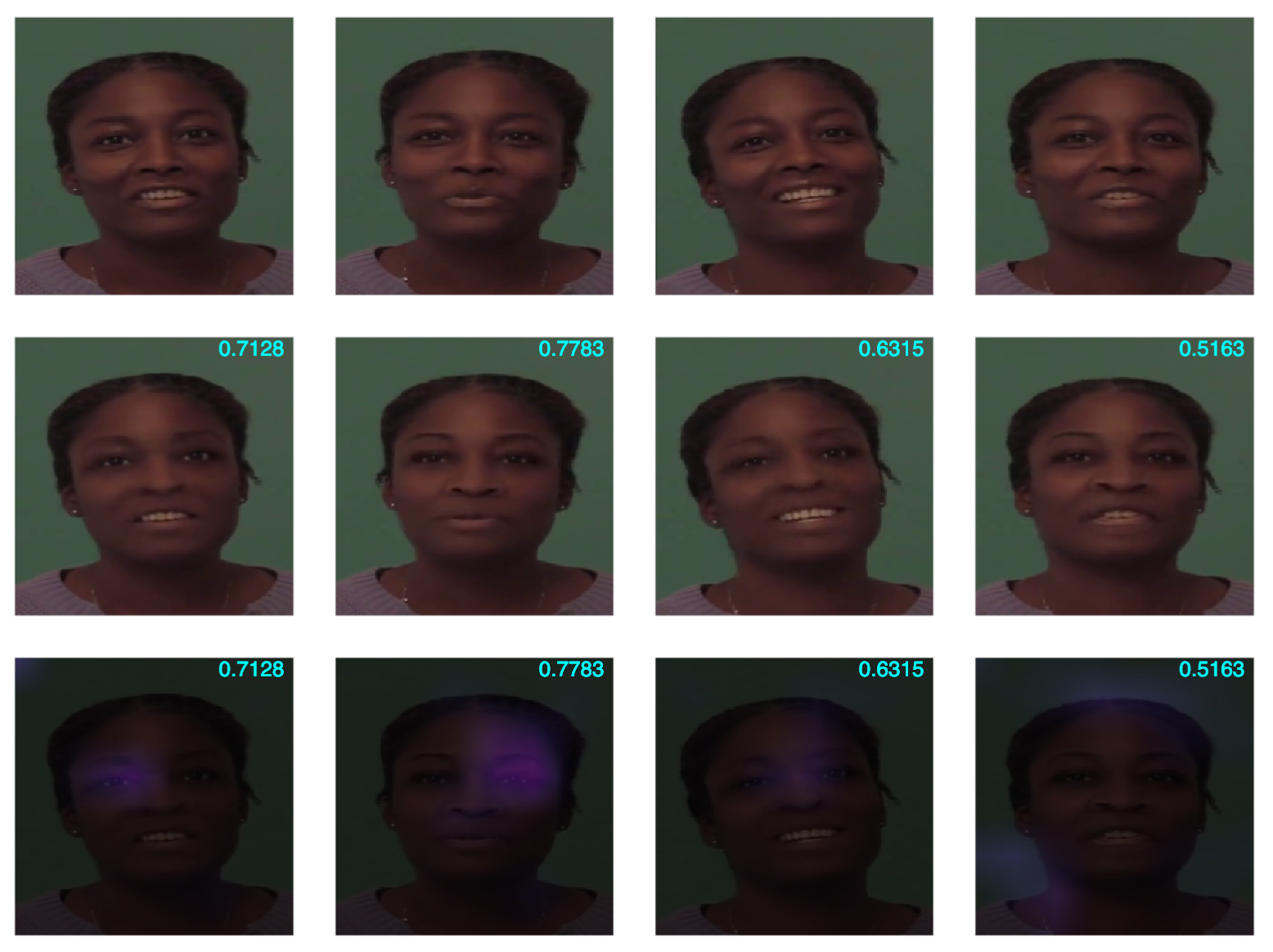
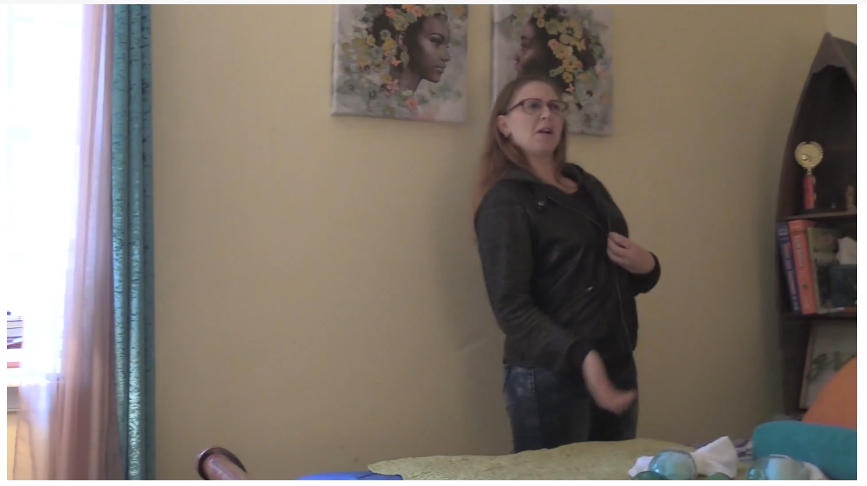
In the next two, final examples, the CAMs plotted don't have the ReLU applied, so they appear brighter in general, but one should still be able to make out where the highlights are. Also, only the deepfake images with CAM overlaid on top are shown.

• Grad-CAM: Why did you say that? Visual Explanations from Deep Networks via Gradient-based Localization

• Learning Deep Features for Discriminative Localization

• CNN Intepretation with CAM, Fastbook